Utility Functions

St. Petersburg Paradox

Consider the following game. A player repeatedly flips a coin. If it lands heads, the player wins 2^0 thalers and leaves the game. If it lands tails, the player flips again, but the potential winnings now are 2^1 thalers. Each subsequent tails doubles the potential winnings.

We can calculate the expected value of the total winnings as follows:

1/2*1 + 1/4*2 + 1/8*4 + ... = inf

In other words, with a probability of 1/2, the player will receive 1 thaler, with a probability of 1/4 (first a tails, then heads) they will receive 2 thalers, with a probability of 1/8 (first two tails, then heads) they will receive 4 thalers, and so on. This series diverges, meaning the expected value of the winnings is infinite.

The subtlety of this game lies in the fact that the player must pay a fee to sit at the game table. The paradox is that although the expected winnings are infinite, people are reluctant to pay even modest amounts.

The paradox was discovered in the early 17th century by a member of the Bernoulli family, and several solutions have been proposed since then. For example, infinite winnings are only possible with an infinite number of games. Considering realistic constraints, both in terms of time and the organizer's capital, the number of games would be finite, making the expected winnings finite.

However, we are interested in a "no-tricks" solution. The chain of reasoning initiated by Daniel Bernoulli led to the development of utility functions by the mid-20th century.

Utility Functions

Bernoulli suggested that the value of money for a player depends on their existing wealth. Clearly, for someone with only 10 thalers, winning 1 thaler is more valuable than it would be for a millionaire. Thus, this win, although having the same monetary value, has different utilities for different players. The function that relates a player's wealth WW to their utility UU is called the utility function.

From the example above, it is intuitively clear that such a function should be concave. For its mathematical description, we can use, for example, the square root or logarithmic function (as Bernoulli did).

Now we see that the player wants to maximize not wealth, but utility. We can calculate the expected value of the utility as follows:

1/2 * (ln(W + 1 - c) - ln(W)) + 
1/4 * (ln(W + 2 - c) - ln(W)) + 
1/8 * (ln(W + 4 - c) - ln(W)) + ... < ∞

Here, W is the player's initial wealth, and c is the fee required to start the game. This sum can be calculated, and it is finite, meaning that for any W, we can compute c. We then find that a millionaire can reasonably play with a fee of 20.88 thalers, a player with 1000 thalers can play with a fee of 10.95 thalers, and a player with 2 thalers should borrow and play for 3.35 thalers. A higher fee makes the game unprofitable in terms of utility.

A Fair Game?

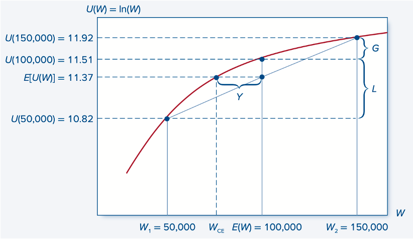
Consider another game. Suppose the player has 100,000 thalers. After flipping a coin, they can either win 50,000 thalers or lose 50,000 thalers. In this sense, we can call the game fair. The expected value of the winnings here is zero, meaning we can expect the player's wealth to remain unchanged over many games.

Now let's look at the situation from a utility perspective. Using a logarithmic utility function, the player's initial utility is 11.51. If they win, it increases to 11.92, and if they lose, it falls to 10.82. Hence, the expected utility (here, the simple average) is only 11.37, which is less than the initial value.

In other words, the potential gain of 50,000 thalers provides less utility to the player than the loss of the same amount detracts.

We can calculate that a utility of 11.37 corresponds to an amount just under 87,000 thalers. Thus, from a utility standpoint, a person with 87,000 thalers is equivalent to a player who can exit the game with either 50,000 or 150,000 thalers. Here, we approach the concept of the importance of risk and the risk premium, which we will discuss in a future post.

Sources: Bodie, Z., & Kane, A. (2020). Investments.